
Communication-efficient Linear Solver Discovery
Introduction
Some of the most important scientific and engineering problems require large-scale computing infrastructure for multi-physics simulations.
We are working on building AI infrastructure to autonomously discover algorithms that speed up these simulations, allowing engineering teams to iterate on designs faster and use higher-fidelity physics models with fewer approximations and higher-order operations for more accurate simulations.
The first domain we are working on is to discover faster linear solvers for simulating the diffusion of the magnetic field through the liner walls of the fusion target inside a magneto-inertial confinement (MagLIF) nuclear fusion device. We built a system to improve the linear solve inside the FLASH multi-physics code that handles the implicit magnetic-diffusion step using the HYPRE library.
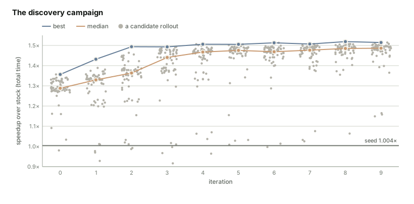
With no access to an actual supercomputing HPC cluster, we simulated a multi-node cluster that models the computing and communication cost of a real cluster as part of the evaluation system of our discovery loop and were able to discover a solver that saves communication overhead in AMG setup by ~49% and achieves an overall speedup of 1.52×.
Background
FLASH is a parallel, adaptive-mesh, multi-physics code [1]. In the magnetic-diffusion problem we target, each implicit step solves one coupled, non-symmetric system for three field components. FLASH solves it using the HYPRE library [2] with a restarted GMRES [4] algorithm that is preconditioned by one V-cycle of BoomerAMG [3]. The multigrid hierarchy is rebuilt for every solve.
AMG has two phases:
- Setup phase: builds a hierarchy of smaller versions of the matrix that includes the coarse grids, the interpolation operators between them, and the coarse operators.
- Solve phase: runs Krylov iterations, each of which applies one V-cycle on all levels of the hierarchy.
At large production scales, the setup phase is the communication-heavy phase and dominates the solver's time-to-solution because each new matrix that is created needs its own communication pattern. Working out the communication pattern requires a round of messages through the multi-node cluster that is expensive.
The goal is to discover solver algorithms that use fewer communication messages without sacrificing accuracy.
Methodology
Simulating an HPC Cluster
A parallel program like FLASH does not run as one copy on one processor but as many copies at once, one per processor core. Each copy, called a rank, owns a slice of the compute. Depending on the algorithm used, every so often the ranks exchange messages using MPI, the standard library that parallel programs use to send messages. A cluster is many separate machines (nodes), each with dozens of cores, joined by a fast network.
Evaluating a solver involves measuring the end-to-end time taken to arrive at a solution on such a multi-node cluster. Renting one for every one of thousands of candidate solvers would have been slow and expensive. So we used SimGrid, an open-source academic toolkit for simulating distributed computer systems [5, 6]. Its MPI part, called SMPI, lets an unmodified MPI program run inside the simulator.
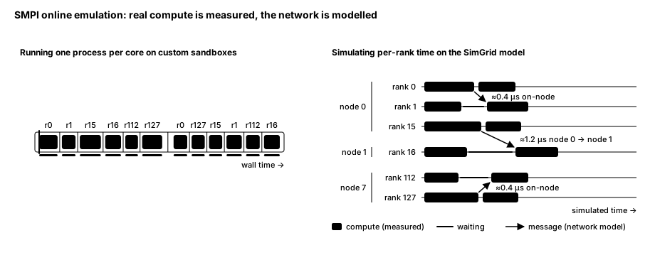
SimGrid runs the program on a simulated cluster:
- All ranks run inside one process, on a single core of a machine. A rank runs until it needs to talk to another rank, at which point SimGrid pauses it and lets another rank continue.
- Each rank has its own clock that shows simulated time, including the compute time spent by that rank.
- When one rank sends data to another, SimGrid simply hands it over in memory. Then a model of the cluster's network works out when the data would have arrived. The model accounts for:
- the delay before the first byte arrives;
- the time needed to push all the bytes through the network's bandwidth;
- the slowdown when several messages share the same bandwidth.
- If a rank needs a message that has not yet "arrived" on the simulated clock, its clock jumps forward to the arrival time. This is similar to how a slow neighbor holds others up on a real cluster.
Example: Simulating a mock 128-rank cluster
Rank 1 computes for 2.000 ms and then sends rank 2 a message, which the network models as 0.005 ms. Rank 2 finished its own work at 1.000 ms and has been waiting for that message. Rank 2's clock therefore jumps to 2.005 ms. In real life rank 2 would have sat idle for a millisecond which our simulation mimics. The solver's time is read from these clocks and measures the wall-clock time taken from the moment all ranks start the solve together to the moment the last one finishes.
The Simulated Cluster
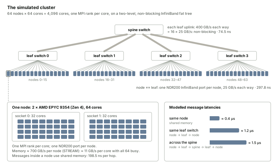
The cluster we simulate is of a common production shape:
- Nodes: 64 nodes with two 32-core AMD EPYC 9354 (Zen 4) processors each, giving us 4,096 cores with one MPI rank per core.
- Memory: about 700 GB/s of bandwidth per node, or about 11 GB/s per core when every core is busy.
- Network ports: one NDR200 InfiniBand port per node, 25 GB/s each way.
- Switches: a two-level, non-blocking fat tree of four leaf switches with 16 nodes each, every leaf joined to the spine by 400 GB/s each way.
- Latency: a small message takes about 0.4 µs within a node, 1.2 µs between nodes on the same leaf and 1.5 µs across the spine.
Simulator time grows roughly with the square of the rank count and even a 1,024-rank run takes more than 90 minutes to finish. This means simulating all 4,096 ranks for every candidate is out of reach for now. So we time each candidate rollout on a quarter-scale version of the cluster.
Dataset
We captured eight systems from multi-rank FLASH runs: four windows of an aluminium-wire (AlWire) setup and four of a Z-pinch (ZPinch) setup. They have 0.93–2.40 million unknowns and each must be solved to a relative residual of 10⁻¹⁰.
Results
BoomerAMG's setup builds a sequence of new distributed hypre_ParCSRMatrix objects: the interpolation operators, the coarse operators using Galerkin triple products and the intermediates of those products. Before a matrix can take part in a matrix–vector or matrix–matrix product, it needs a communication package (hypre_ParCSRCommPkg) that includes its neighbor ranks, the off-processor columns to receive from each rank (the matrix's col_map_offd) and the local rows to send to each rank. A rank knows only which global columns its off-diagonal block references, not which ranks own them or which ranks need its own rows. So hypre_MatvecCommPkgCreate discovers the pattern at run time with two rounds of hypre_DataExchangeList which is a sparse data exchange. In the first round, each rank asks the owner of every column range it needs under HYPRE's assumed partition of the global index space [7] which ranks actually hold those columns. In the second, it sends each actual owner the list of columns it needs, and the owners assemble their send maps from these requests.
- Every rank sends its queries, then spins on
MPI_IprobeandMPI_Testuntil a termination signal travels through a tree over all 128 ranks. - Each exchange therefore behaves like a global barrier, and the polls count time spent waiting for the slowest rank.
The winning solver reduced AMG setup time by ~49%. Against the stock, the winner's setup:
- sends 0.35× the bytes, and 0.32× across nodes;
- polls 0.43× as often (36 million → 16 million polls over all ranks and matrices);
- makes half as many MPI calls;
- spends 0.53× as long blocked in MPI.
References
- B. Fryxell, K. Olson, P. Ricker, F. X. Timmes, M. Zingale, D. Q. Lamb, P. MacNeice, R. Rosner, J. W. Truran, H. Tufo. “FLASH: An Adaptive Mesh Hydrodynamics Code for Modeling Astrophysical Thermonuclear Flashes.” The Astrophysical Journal Supplement Series 131(1):273–334, 2000.
- R. D. Falgout, U. M. Yang. “hypre: A Library of High Performance Preconditioners.” In Computational Science — ICCS 2002, Part III, Lecture Notes in Computer Science 2331, pp. 632–641. Springer, 2002.
- V. E. Henson, U. M. Yang. “BoomerAMG: A parallel algebraic multigrid solver and preconditioner.” Applied Numerical Mathematics 41(1):155–177, 2002.
- Y. Saad, M. H. Schultz. “GMRES: A Generalized Minimal Residual Algorithm for Solving Nonsymmetric Linear Systems.” SIAM Journal on Scientific and Statistical Computing 7(3):856–869, 1986.
- A. Degomme, A. Legrand, G. S. Markomanolis, M. Quinson, M. Stillwell, F. Suter. “Simulating MPI Applications: The SMPI Approach.” IEEE Transactions on Parallel and Distributed Systems 28(8):2387–2400, 2017.
- H. Casanova, A. Giersch, A. Legrand, M. Quinson, F. Suter. “Versatile, scalable, and accurate simulation of distributed applications and platforms.” Journal of Parallel and Distributed Computing 74(10):2899–2917, 2014.
- A. H. Baker, R. D. Falgout, U. M. Yang. “An assumed partition algorithm for determining processor inter-communication.” Parallel Computing 32(5–6):394–414, 2006.